Annotations
Due by 11:59 PM on Monday, October 23, 2023
For this exercise, you’ll use whatever data you want to make a plot and add annotations to it. Use a dataset from a past exercise, use one of the built-in datasets like mpg or gapminder from the {gapminder} package, download stuff from the World Bank using the {WDI} package, or use something from this list of datasets.
This example page will be incredibly useful for you:
You’ll be doing all your R work in R Markdown. You can download a zipped file of a pre-made project here:
You don’t need to make your plots super fancy (except for these annotations), but you should play around with the plots and try to go beyond the basics—experiment with changing colors or modifying themes and theme elements.
And as always, if you’re struggling, please talk to me and use Slack and talk to your classmates! Don’t suffer in silence!
Instructions
If you’re using R on your own computer, download this file, unzip it, and double click on the file named
exercise-9.Rproj:09-exercise.zipYou’ll need to make sure you have the
tidyversepackage installed on your computer. If you try to load it withlibrary(tidyverse)and R gives an error that the package is missing, use the “Packages” panel in RStudio to install it.(Alternatively, you can open the project named “Exercise 9” on Posit.cloud and complete the assignment in your browser without needing to install anything. This link should take you to the project—if it doesn’t, log in and look for the project named “Exercise 9”.)
Rename the R Markdown file named
your-name_exercise-9.Rmdto something that matches your name and open it in RStudio.Complete the tasks given in the R Markdown file.
Fill out code in the empty chunks provided (you can definitely copy, paste, and adapt from other code in the document or the example page—don’t try to write everything from scratch!).
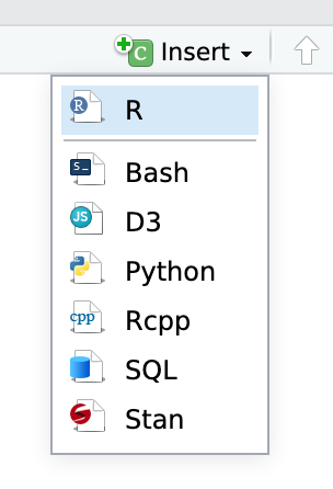
You’ll need to insert your own code chunks. Rather than typing them by hand (that’s tedious!), use the “Insert” button at the top of the editing window, or press ⌥ + ⌘ + I on macOS, or ctrl + alt + I on Windows.
Remember that you can run an entire chunk by clicking on the green play arrow in the top right corner of the chunk. You can also run lines of code line-by-line if you place your cursor on some R code and press ⌘ + enter (for macOS users) or ctrl + enter (for Windows users).
Make sure you run each chunk sequentially. If you run a chunk in the middle of the document without running previous ones, it might not work, since previous chunks might do things that later chunks depend on.
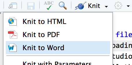
When you’re all done, click on the “Knit” button at the top of the editing window and create a Word or PDF version (if you’ve installed tinytex) of your document. Upload that file to iCollege. Do not upload a knitted HTML file (they don’t work on iCollege).